Backpropagation: one backwards pass that trains a whole network

What backpropagation is

Training a neural network means nudging millions of settings (called weights) so that its error gets smaller. To do that, you need to know, for every single setting, which way to nudge it and by how much. Backpropagation is the method that answers that question for all of them at once.

It starts at the error and walks backwards through the calculation, towards the inputs, handing each step its share of the responsibility. Under the hood it is the chain rule from calculus, run in reverse: multiply the rates of change along each path, and add up the paths whenever a value is used in more than one place.

What the video shows

The video points to an imbalance: a network has millions of settings but only one error. Walking backwards from that error a single time tells you how every setting contributed, at roughly the cost of computing the error in the first place.

An everyday example

Imagine a company that closes the quarter with a loss and wants to know how much each of its 1,000 employees' decisions contributed. One way is to replay the whole quarter 1,000 times, changing one person's decision each time. The other is to start from the final number and walk back through the organisation once: the board passes responsibility down to departments, departments to teams, teams to people, and each level works out its own share from what the level above handed down.

The second approach is backpropagation. Working forwards would take one full pass per setting. Working backwards takes one pass in total. With millions of settings, that difference is what makes training large models practical at all.

A worked example from the course

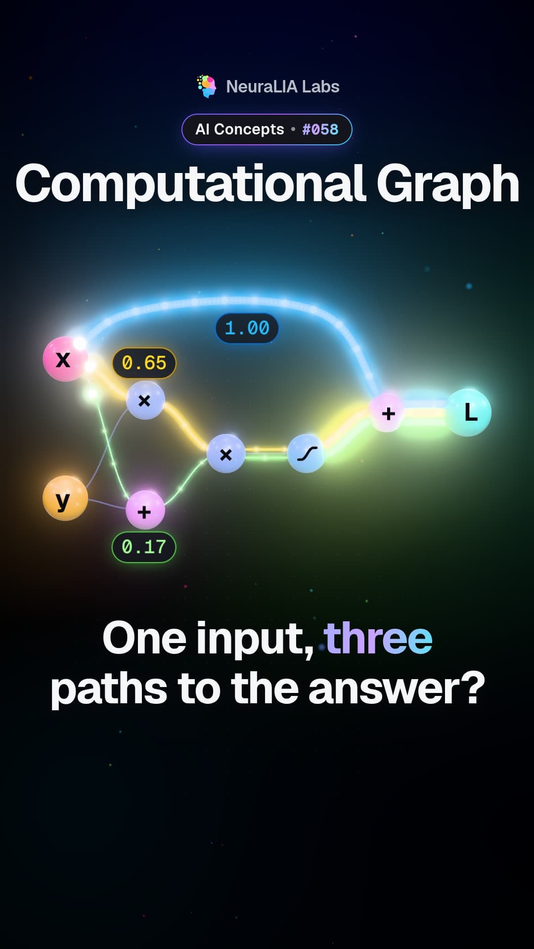
The course does this by hand on a tiny calculation with five steps, starting from x = 0.5 and y = 1.4:

• a = x × y = 0.7
• b = x + y = 1.9
• c = a × b = 1.33
• d = tanh(c), a curve that squashes numbers into a fixed range
• final result L = d + x

Notice that x is used three times. Walking backwards from L gives three separate paths to x, and each one contributes:

| Path from the result to x | Contribution | |---|---| | through a | 0.6501 | | through b | 0.1711 | | directly into L | 1.0000 | | Total | 1.8212 |

So nudging x up by a tiny amount raises the result by about 1.82 times that amount. Later in the chapter, a program of about 120 lines works out the same 1.8212 on its own, and agrees with PyTorch, a widely used AI toolkit, to within roughly 0.0000000000000002.

A bit of history

The method was popularised in 1986. It answered the question that the researchers Minsky and Papert had left open: how do you train a network made of several layers stacked on top of each other? Without a way to share out the responsibility across layers, deeper networks could be built but not taught.

Why it matters

Backpropagation is the step that makes training giant networks possible. The idea fits in one sentence (multiply along each path, add across paths), yet it turns an impossible amount of trial and error into a single backwards sweep. Understanding it also demystifies what "training" means: nothing more magical than careful, repeated blame assignment.

Learn it step by step in Chapter 5 of our free course AI From Scratch: Backpropagation From Scratch: The Engine, Then the Network.